WSC 2023: Persistent low physical activity after stroke and risk of new vascular event or death

Here is a few background notes on my oral presentation at the World Stroke Congress 2023.

Intro

I will presenting our work on “Persistent low physical activity after stroke and risk of new vascular event or death” at the World Stroke Congress 2023, Toronto, Canada on 11 October.

I intended to do a little write up of the preparation work and the data analyses. Now, at the conference, I will be presenting tomorrow, and this is the last chance to put my notes together.

A long-term, registry based follow-up

Our study is based on the [TALOS-trial](https://www.doi.org/10.1161/STROKEAHA.117.020067) cohort,. The trial was a randomised trial on citalopram in acute ischaemic stroke conducted between 2013-2016. For this study we did long-term follow-up on the pre-defined composit outcome of new vascular event (stroke, TIA or MI) or death of any cause. These data were obtained through the Danish health registries, that are based on a civil registration number given to all people living in Denmark. We have had access to hospital admission data nd death registrations. When sending in the abstract for WSC, I expected we would have been able to enrich our dataset further with data on socio-economic status as well as educational level. We are still awaiting these data, however, but these will be included when we get to the final publication of our findings.

Main points presented

At the WSC I will be presenting two of our main findings:

1. Patients with a persistent low level of physical activity (in the lowest quartile of our physical activity score measure) at both seven days just prior to their stroke as well as six months post-stroke have a significantly increased hazards ratio (HR) of our composite outcome, compared to the group of patients in the 2nd-4th quartile at both pre-stroke and six months post-stroke.
2. Patients in the lowest quartile pre-stroke, but in one the the higher quartile post-stroke, did not have a HR statistically significantly different from the group with a higher level at both time points.

I think the first point is what we expected, but the second point is very encouraging. Though, this trial is observational, it still highlights, that increasing physical activity level in the stroke population may lower the risk of a clinical outcome such as new vascular event or death.

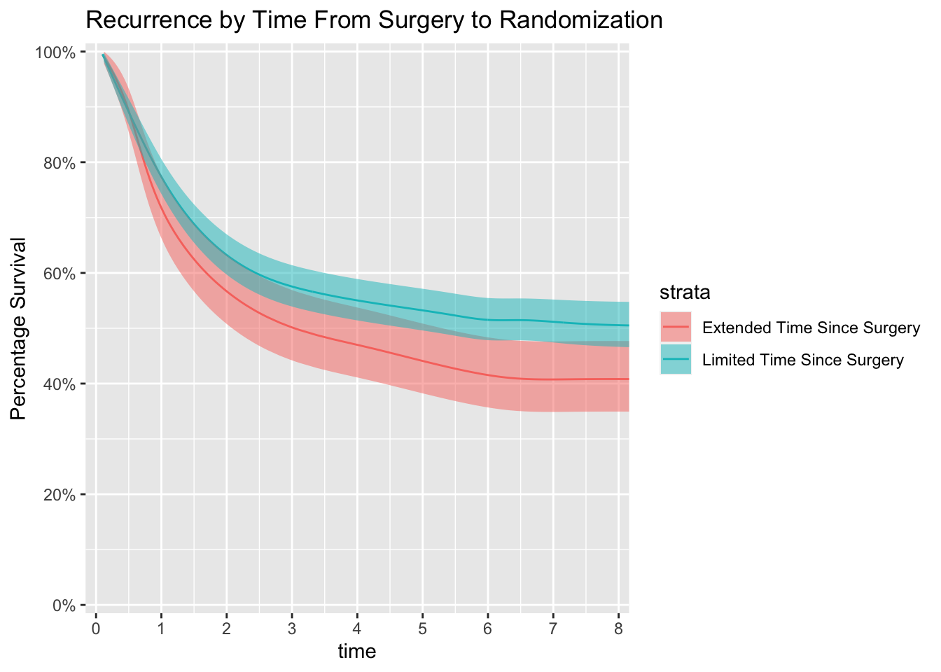
Smoothed survival plot

I have been quite restricted in data management and which figures to present, as I have been working on a protected server, and I have only been allowed to present cumulative data. This means, that I also had to find a way to smooth the classic survival curve plot, as each step on the classic plot is representing a single subject, and thereby not allowed.

Below is the code I used for my presentation at WSC with some sample data. This code is based on the `ggsurvfit`-package, which eases the work with survival data, but I had to use a different approach to the smooth line and confidence interval. I played with other smoothing approaches, but this is the most straight-forward, I found.

library(tidyverse)

── Attaching core tidyverse packages ──────────────────────── tidyverse 2.0.0 ──
✔ dplyr     1.1.3     ✔ readr     2.1.4
✔ forcats   1.0.0     ✔ stringr   1.5.0
✔ ggplot2   3.4.3     ✔ tibble    3.2.1
✔ lubridate 1.9.3     ✔ tidyr     1.3.0
✔ purrr     1.0.2     
── Conflicts ────────────────────────────────────────── tidyverse_conflicts() ──
✖ dplyr::filter() masks stats::filter()
✖ dplyr::lag()    masks stats::lag()
ℹ Use the conflicted package (<http://conflicted.r-lib.org/>) to force all conflicts to become errors

library(survival)
library(purrr)
library(ggsurvfit)

df <- survfit2(Surv(time, status) ~ surg, data = df_colon) |> 
  tidy_survfit(type = "survival")

df_split <- split(df,df$strata)

df_smoothed <- purrr::reduce(lapply(c("estimate","conf.low", "conf.high"), function(j) {
  do.call(rbind,
          lapply(seq_along(df_split), function(i) {
            nms <- names(df_split)[i]
            y <-
              predict(mgcv::gam(as.formula(paste0(
                j[[1]], " ~ s(time, bs = 'cs')"
              )), data = df_split[[i]]))
            df <- data.frame(df_split[[i]]$time, y, nms)
            names(df) <- c("time", paste0(j[[1]], ".smooth"), "strata")
            df
          }))
}),dplyr::full_join) |> full_join(df)

Joining with `by = join_by(time, strata)`
Joining with `by = join_by(time, strata)`
Joining with `by = join_by(time, strata)`

ggplot(data=df_smoothed) +
  geom_line(aes(x=time, y=estimate.smooth, color = strata))+
  geom_ribbon(aes(x=time, ymin = conf.low.smooth, ymax = conf.high.smooth, fill = strata), alpha = 0.50) +
  # geom_smooth(aes(x=time, y=estimate, color = strata), method = "gam", formula = y ~ s(x, bs = "cs")) +
  # reduce padding on edges of figure and format axes
  scale_y_continuous(label = scales::percent, 
                     breaks = seq(0, 1, by = 0.2),
                     expand = c(0.015, 0), limits = c(0,1)) +
  scale_x_continuous(breaks = 0:10, 
                     expand = c(0.02, 0))+
  labs(
    y = "Percentage Survival",
    title = "Recurrence by Time From Surgery to Randomization",
  ) +
  # limit plot to show 8 years and less
  coord_cartesian(xlim = c(0, 8))

Warning: Removed 9 rows containing missing values (`geom_line()`).